VLOOKUP, HLOOKUP, XLOOKUP

VLOOKUP in Excel: find a price by product code

VLOOKUP is the quickest way to bring a value from one table into another: a price list on the left, orders on the right, and the price filled in by product code. Type the formula, copy it down, and rows without a match show a clear message instead of an error.

Exact and approximate match
Argument hints
Free
No sign-up

How to use VLOOKUP step by step

VLOOKUP: price list and orders
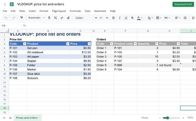
Open the example: a price list of eight products with code, name and price on the left, and orders on the right. Each order has a product code, and the price column is filled in from the list.
Formula bar
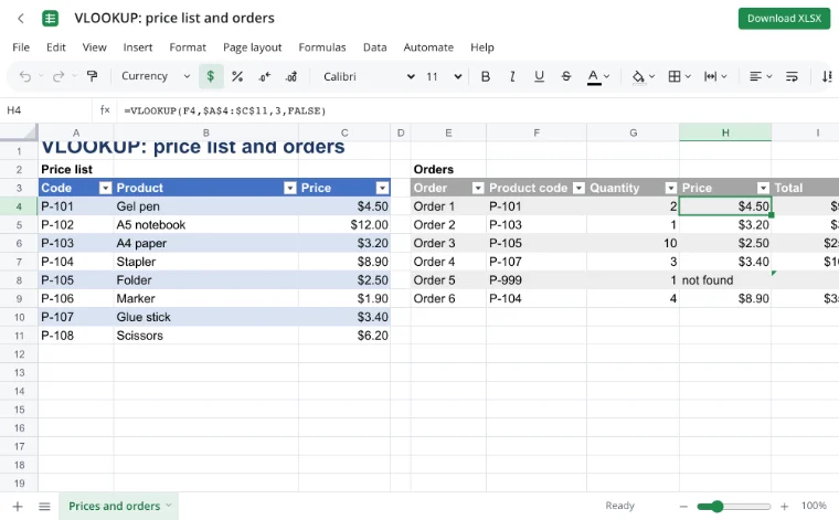
Select the price cell in the first order and enter =VLOOKUP(F4,$A$4:$C$11,3,FALSE) in the formula bar. F4 is the code, A4:C11 the price list, 3 the price column, and FALSE asks for an exact match.
Fill handle
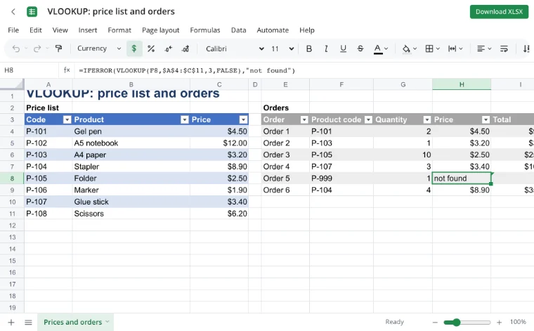
Drag the formula down with the fill handle. The $ signs keep the price list fixed while each row looks up its own code. In the example, an order with an unknown code is wrapped in IFERROR and shows “not found”.

Everyday work

Use cases

A supplier price list and a purchase order: the code sits in the order, the price comes from the list.
A CRM export and an invoice list: match a customer ID to a company name.
Payroll: pull a tax rate or an hourly rate from a reference table by code.
A school grade sheet: bring a student's name or grade from a roster by ID.
E-commerce: fill product names and prices into an order export.

Formula

How do I use VLOOKUP in Excel?

VLOOKUP takes four arguments: the value to find, the range to search, the column number to return, and the match type. It looks for the value in the first column of the range and returns the value from the same row in the column you name.

Write =VLOOKUP(F4,$A$4:$C$11,3,FALSE) to find the code in F4 and return the third column — the price. FALSE means an exact match.

First argument — the value to find: a product code, SKU or ID.
Second — the range whose first column holds the same codes.
Third — the column number in that range to return; the price is column 3 in the example.
Fourth — FALSE for an exact match, TRUE for an approximate one.

Two sheets

How do I use VLOOKUP between two sheets?

Put the lookup range on the other sheet and prefix it with the sheet name: =VLOOKUP(F4,Prices!$A$4:$C$11,3,FALSE). The rest of the formula stays the same. If the sheet name contains a space, wrap it in single quotes, as in 'Price list'!$A$4:$C$11.

XLOOKUP

What is the difference between VLOOKUP and XLOOKUP?

XLOOKUP is more flexible: it searches any column, returns a value from any column, matches exactly by default and accepts an “if not found” argument. VLOOKUP searches only the first column and returns values to the right. Both work here, and the example uses XLOOKUP for one order so you can compare the results.

Matching

Exact match, approximate match and wildcards

Use FALSE for codes and IDs: an exact match is what you almost always need. TRUE finds the nearest lower value in a sorted first column, which suits tax brackets or discount tiers. Wildcards * and ? work in exact text matches, so “*delivery*” finds a code containing that word, and matching ignores letter case.

Features

Feature	What it gives you
VLOOKUP	Exact and approximate match, wildcards and case-insensitive text.
HLOOKUP	The same lookup across the first row instead of the first column.
XLOOKUP	Any column order, exact match by default and an “if not found” value.
INDEX and MATCH	A lookup pair for ranges where the key is to the right of the result.
IFERROR and IFNA	Turn #N/A into “not found” or another readable message.
Argument hints	The editor shows what each argument expects while you type.

Limits

VLOOKUP searches only the first column of the range and returns values to its right.
Approximate match needs the first column sorted in ascending order.
VBA macros do not run, and the old binary XLS format does not open.
Real-time co-editing is not available.

Privacy

The workbook is opened and calculated in your browser, so a price list or a payroll reference stays on your device. It reaches a server only through “Save to cloud”, and cloud files are stored in the EU/US under GDPR. A finished sheet can go out as a PDF through the Excel to PDF converter.

Frequently asked questions

Support: [email protected]

How to use VLOOKUP?

Write =VLOOKUP(value, range, column, FALSE). The value is what you look for, the range must have that value in its first column, the column number says what to return, and FALSE asks for an exact match. Press Enter and drag the formula down. If nothing matches, wrap it in IFERROR to show a readable message.

How to VLOOKUP?

Start the formula with =VLOOKUP and four arguments separated by commas. Anchor the range with $ signs so it does not move when you copy the formula. Use FALSE for codes and IDs. To look up a value on another sheet, put the sheet name before the range, as in Prices!$A$4:$C$11.

How to VLOOKUP in Excel?

Select the result cell, type =VLOOKUP(, and fill in the code, the range, the column number and FALSE. The editor shows the arguments as you type. This works the same way as in Excel: the formula reads the first column of the range and returns a value from the same row to the right.

How to use VLOOKUP in Excel?

Use it when two tables share a key: an order code, an employee ID or a SKU. Put the key in the first column of the lookup range, write the formula in the table that needs the extra value, and copy it down. For a missing key, add IFERROR so the cell shows “not found” instead of #N/A.

How to use VLOOKUP in sheets?

The formula is the same in this browser editor: =VLOOKUP(F4,$A$4:$C$11,3,FALSE). Open the example to see a price list and orders, select the price cell and copy the formula down. Nothing is installed, and the file stays on your device until you save it to the cloud.

How to use VLOOKUP in Excel between 2 sheets?

Write the range with the sheet name: =VLOOKUP(F4,Prices!$A$4:$C$11,3,FALSE). The first column on that sheet must hold the codes you search for. If the name has a space, use single quotes around it. The rest of the arguments do not change.

How to use VLOOKUP and XLOOKUP together?

Use VLOOKUP for simple lookups to the right of the key, and XLOOKUP when the result column is to the left, when you need a value for a missing key, or when you want to search from the end. Both return the same value for a straightforward code match, so you can compare them in one sheet.

Is it free? Is there a watermark?

Yes, the tool is free: no payment, trial period or watermark. All lookup functions and argument hints are available at once, and no account is needed to open a workbook, calculate a formula and download the file. Signing in is only required to keep a workbook in the cloud.

Is it safe to upload documents?

Nothing is uploaded: the workbook is opened and calculated in your browser on your own device. Price lists, orders and payroll references therefore stay with you. A file reaches a server only if you choose “Save to cloud” and sign in, and then it is stored in the EU/US under GDPR.