Rulesscales · icons

Conditional formatting: highlight the cells that need attention

Conditional formatting changes a cell's look when its value meets a rule, so a sales sheet or a budget shows problems without anyone repainting rows by hand. Set the condition once in “Format”, and the color, bar or icon appears whenever the numbers cross the line.

Value and formula rules
Data bars and color scales
Free
No sign-up

How to use conditional formatting

“Conditional formatting” example
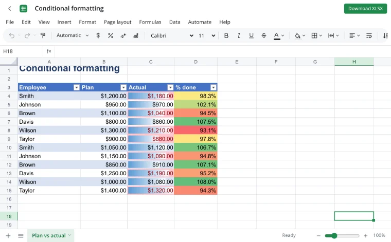
The example sheet has a target column, an actual revenue column and a completion percentage. A three-color scale runs down the percentage, data bars sit inside the actual column, and rows below target carry light red fill with dark red text.
“Manage rules”
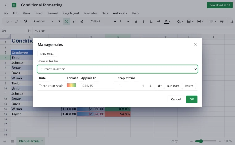
“Manage rules” lists every rule on the selected range or on the whole sheet. Change, duplicate, delete or reorder rules here, switch on “Stop if true” and edit the range a rule applies to.
“Format ▸ Conditional formatting”
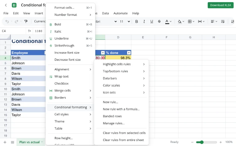
The “Format ▸ Conditional formatting” menu opens the ready-made sets: highlight cells rules, top/bottom rules, data bars, color scales and icon sets. The quick analysis button next to a selection offers the same choices.
“New rule with a formula”
For your own condition choose “New rule…” or “New rule with a formula”. The formula returns true or false, and references start from the top-left cell of the range — =C4<B4 colors the rows where actual revenue is below target.

Rule types

What conditional formatting can do

Rule	What it does
Highlight cells rules	Greater, less, between, equal, text contains, a date, duplicates.
Top/bottom rules	Top or bottom 10 items, top or bottom percent, above or below average.
Data bars	A bar inside the cell shows size next to the number.
Color scales	Two- or three-color gradient from the lowest to the highest value.
Icon sets	Arrows, traffic lights, flags and stars instead of hand-made marks.
Formula rule	Your own condition that can read other columns or cells.
Banded rows	Alternating fill that makes long tables easier to follow.
Manage rules	Rule order, duplicates, “Stop if true” and the range a rule covers.

Step by step

How to apply conditional formatting in Excel

Select the cells, open “Format ▸ Conditional formatting” and choose a set. Highlight cells rules cover numbers, text, dates, blanks and duplicates; top/bottom rules find the largest or smallest values; data bars, color scales and icon sets add a visual layer without changing the numbers.

For a condition of your own, open “Manage rules” or “New rule with a formula”. The rule is written into the workbook, so a sheet highlighted here keeps its colors when it is opened in Excel. Zotu is not affiliated with Microsoft; it is a separate editor that reads and writes Excel files.

Formulas

Rules that follow another cell

A formula rule decides the format from any cell, not only the one being colored. Select the rows you want to mark, choose “New rule with a formula” and write =C4<B4, where references start from the top-left cell of the selection. Lock the column with $ when every row should compare against the same cell.

If the cutoff lives in a single cell, point the rule at it — the rule reads that value and updates when it changes. Test the expression in a cell first: when it returns true, the highlight will fire. More on writing conditions and references is in formulas.

Everyday checks

Dates, blanks and duplicates

The date rules cover today, yesterday, tomorrow, the last seven days, this month and dates that have passed, which makes an invoice or application tracker readable at a glance. Blank cells have their own rule, and “Duplicate values” finds repeated order numbers, emails or phone numbers in the selected range. None of these needs a formula.

Use cases

Everyday uses

Invoices: a due date that has passed turns red.
Sales targets: rows below quota are filled, rows above quota are green.
Budget: a color scale shows which categories are running hot.
Inventory: stock below the reorder point gets an icon.
College applications: deadlines in the next week stand out.
Customer lists: duplicate emails are easy to spot before a mail merge.

Outlook

What conditional formatting in Outlook means

Conditional formatting in Outlook is a mail feature that highlights messages in the inbox by sender, subject or date. It is separate from spreadsheet rules and is not part of this editor. The rules described on this page apply to cells in a workbook: values, formulas, dates, bars, scales and icons.

Devices

On a phone and on a laptop

Rules can be set in a mobile browser on Android and iPhone, and the result is easy to read on a small screen. A long list of rules, overlapping ranges and their order are easier to review on a laptop, where the dialog and the sheet fit side by side.

Limits

Real-time co-editing is not available: two people cannot edit one workbook at once.
VBA macros do not run; an XLSM file is saved as XLSX.
The older XLS format does not open, and workbooks with an open password are not supported.
On the tool page a file is limited to 100 MB.

Privacy

The workbook opens and recalculates in your browser on your own device, so targets, payroll and customer lists stay with you. A file reaches a server only through “Save to cloud”, and cloud files are stored in the EU/US under GDPR. A highlighted sheet can be saved as a PDF or shown as a chart.

Frequently asked questions

Support: [email protected]

How do I apply conditional formatting in Excel?

Select the cells, open “Format ▸ Conditional formatting” and pick a ready-made set: highlight cells, top/bottom, data bars, color scales or icon sets. For your own condition choose “New rule…” or “New rule with a formula”. The rule applies to the selected range at once and is saved with the workbook.

How do I use conditional formatting based on another cell?

Use a formula rule and point it at the other cell. Select the range to color, choose “New rule with a formula” and write a condition such as =C4<B4, where the references start from the top-left cell. Lock the column with $ when every row should compare against the same cell.

How do I format dates with conditional formatting?

Date rules live under “Highlight cells rules ▸ A date occurring”. They cover today, yesterday, tomorrow, the last seven days, this month and dates that have passed. For a fixed cutoff, write a formula rule that compares the cell with TODAY() or with a date in another cell. Blank cells have a rule of their own.

How do I highlight an entire row based on one cell?

Select the whole row range, then create a formula rule whose condition reads the key cell, for example =$D4<0. The dollar sign keeps the column fixed while the row number moves down the selection, so each row is judged by its own value in column D. Apply the rule to every row you want colored.

Can I copy conditional formatting to other cells?

Open “Manage rules”, duplicate the rule and set a new range under “Applies to”, or simply change the range of the existing rule. Copying cells carries the rule with them. Check relative references afterwards: they count from the new top-left cell and may point at the wrong column.

How do I remove conditional formatting?

Select the cells and open “Manage rules”, then delete the rule you no longer need. “Clear rules from selected cells” removes every rule on the selection, and “Clear rules from entire sheet” removes them all. Fill and font applied by hand stay in place; only the automatic highlighting disappears.

Is it free? Is there a watermark?

Yes, every part is free: rules, data bars, color scales, icon sets and rule management work without payment, a trial period or a watermark. You can open a workbook and set up highlighting without an account. Signing in is needed only to keep the file in the cloud.

Is it safe to upload documents?

Nothing is uploaded: the workbook opens and recalculates in your browser on your own device, so targets, payroll and customer lists stay with you. A file reaches a server only through “Save to cloud”, and cloud files are stored in the EU/US under GDPR.