Sortfilter · totals

Filter in Excel: sort rows and keep only the records you need

Filtering in Excel is the quickest way to shrink a long list to the rows that matter: unpaid invoices, applicants at one stage or orders from a single state. Turn on the filter buttons, tick the values you want and the rest of the sheet steps aside without being deleted.

Sort A→Z and Z→A
Filter by value, color or condition
Free
No sign-up

How to filter and sort a table

“Sort and filter” example
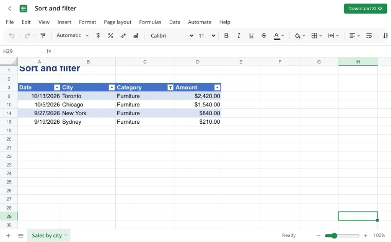
The example holds sales rows with a date, city, category and amount. It opens sorted by amount from largest to smallest, and a category filter is already on, so only one category is visible on the sheet.
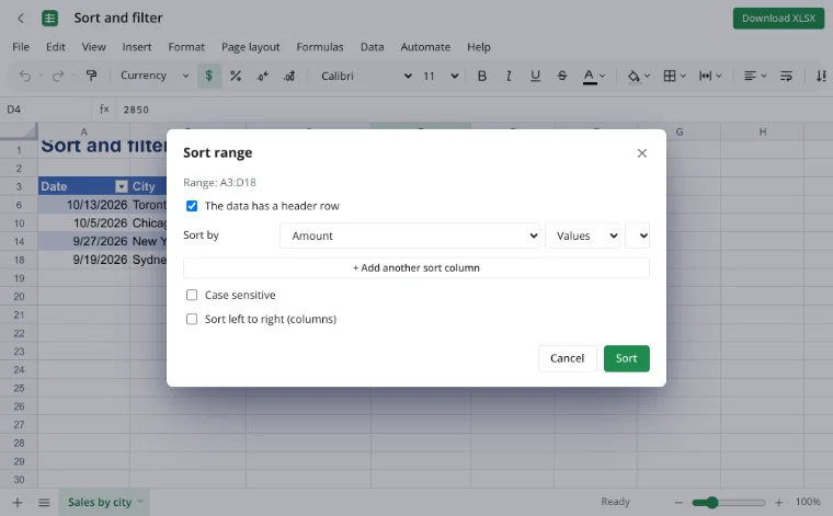
“Sort range…”
“Sort range…” sets several levels and asks whether the range has a header row. Rows can be ordered by value, cell color or font color, and the header stays at the top.
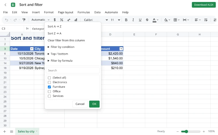
Column menu
The arrow in a header opens the column menu: “Sort A → Z”, “Sort Z → A”, “Clear filter”, “Filter by condition”, “Top / bottom”, “Filter by formula” and “Filter by color”. Below it sit the search box and the value list with “Select all”.
“Data ▸ Filter”
Turn the buttons on with “Data ▸ Filter” or Ctrl+Shift+L. Smart tables show them by default, and Alt+↓ opens the column menu from the keyboard.

Filtering

How to filter in Excel

Click a cell inside the table and choose “Data ▸ Filter” or press Ctrl+Shift+L. Arrows appear in the header row. Open the menu of one column and either tick values from the list or set a condition such as greater than, between or contains.

Conditions in different columns work together: a city and a category can be active at the same time. To drop one condition, use “Clear filter” in that column; to remove every arrow, switch the filter off again with the same command or shortcut.

Sorting

Sort data in Excel without breaking rows

Click a cell in the table and use “Sort A → Z” or “Sort Z → A”. The editor detects the header row and moves whole rows, so an amount never slides over to a different order. For more than one level, open “Sort range…”, add the second and third columns and confirm that the range has a header.

Sorting a single column while its neighbors stay put breaks the table: values no longer belong to their row. Sort the whole range or a smart table instead, and keep the header in one row with no blank rows inside the data.

Reference

The column menu, item by item

Item	What it does
Sort A → Z / Z → A	Orders whole rows by the column and keeps the header in place.
Clear filter	Brings back the rows hidden by this column.
Value list and search	Ticks values one by one; “Select all” restores the column.
Filter by condition	Greater, less, between, contains and similar rules.
Top / bottom	The highest or lowest values in the column.
Filter by formula	A condition written as an expression.
Filter by color	Keeps rows by fill or font color.
Data ▸ Filter	Shows or hides the filter buttons for the range.
Alt+↓	Opens the column menu from the keyboard.

Several conditions

Filter in Excel with multiple criteria

Each column keeps its own filter, and the visible rows must satisfy all of them. That makes a narrow question easy: state equals New York, status equals open and amount greater than 5000 leaves exactly the rows that match every condition. The menu shows a filter icon on every active column, so it is clear where the narrowing comes from.

Advanced filters

Filter by condition, color and formula

“Filter by condition” covers comparisons that a value list cannot express, and “Top / bottom” keeps the largest or smallest entries. “Filter by color” reads the fill or font color, which pairs well with cells already marked by conditional formatting. “Filter by formula” is the escape hatch for a rule that spans several columns.

Use cases

Accounts receivable: open invoices past their due date.
Hiring: applicants at the interview stage, sorted by application date.
Expenses: transactions above a limit for one month.
E-commerce: orders from one country, largest first.
Inventory: SKUs below the reorder point.
Events: registrations sorted alphabetically by last name.

Totals

Totals on visible rows only

A filter hides rows; it does not delete them. SUBTOTAL and AGGREGATE count only the visible rows, so a sum under the table ignores what the filter has hidden. If you need a separate summary instead of a narrowed view, build a pivot table or clean the export first with the CSV converter.

Shortcuts

Shortcuts and smart tables

Ctrl+Shift+L turns the filter buttons on and off.
Alt+↓ opens the menu of the current column.
A smart table keeps its filter buttons and grows with new rows.
Header names must sit in one row, with no blank rows inside the data.

Limits

Real-time co-editing is not available: two people cannot edit one workbook at once.
VBA macros do not run; an XLSM file is saved as XLSX.
The older XLS format does not open, and workbooks with an open password are not supported.
On the tool page a file is limited to 100 MB.

Privacy

The workbook opens and calculates in your browser on your own device, so sales exports, bank transactions and applicant lists stay with you. A file reaches a server only through “Save to cloud”, and cloud files are stored in the EU/US under GDPR.

Frequently asked questions

Support: [email protected]

How do I filter in Excel?

Click a cell in the table and choose “Data ▸ Filter” or press Ctrl+Shift+L. Arrows appear in the header row. Open the menu of the column you need and tick values from the list or set a condition. Conditions in several columns work together, and the hidden rows stay in the workbook.

How do I sort data in Excel by date?

Select a cell in the table and use “Sort A → Z” or “Sort Z → A” on the date column; the editor recognizes the header and moves whole rows. For a second level, open “Sort range…” and add another column. Dates must be real date values, not text, or the order will follow the characters.

How do I filter in Excel with multiple criteria?

Turn on the filter buttons and set a condition in each column you need. The visible rows must satisfy all of them, so a state, a status and an amount can narrow the list together. Active columns show a filter icon. Use “Clear filter” in one column to relax just that condition.

How do I filter in Excel by column?

Switch on “Data ▸ Filter”, then click the arrow in the header of that column. The menu offers sorting, a value list with search, “Filter by condition”, “Top / bottom”, “Filter by formula” and “Filter by color”. Alt+↓ opens the same menu from the keyboard.

How do I clear a filter in Excel?

Open the column menu and choose “Clear filter” to bring back the rows hidden by that column. To remove every arrow from the range, choose “Data ▸ Filter” again or press Ctrl+Shift+L. Clearing a filter never deletes rows; it only shows them again.

How do I filter and delete rows in Excel?

A filter hides rows rather than deleting them, so first narrow the list to the records you want to remove. Select the visible rows, delete them, then clear the filter. Check the total row afterwards: formulas that count visible rows change as soon as the hidden ones are gone for good.

Is it free? Is there a watermark?

Yes, sorting, filtering, conditions and totals are free, with no trial period and no watermark. You can open a workbook and narrow a list without an account. Signing in is needed only for cloud storage, and a filtered sheet can be downloaded at any time.

Is it safe to upload documents?

Nothing is uploaded: the workbook opens and calculates in your browser on your own device, so sales exports, bank transactions and applicant lists stay with you. A file reaches a server only through “Save to cloud”, and cloud files are stored in the EU/US under GDPR.